Lab 5: Raster Modeling

Goal 

This lab worked to build models for frac sand mining suitability and frac sand mining impact for Trempealeau County, WI by using a variety of raster geoprocessing tools.  The two models were then overlaid to determine the best overall locations for frac sand mines in Trempealeau County.  The impact of sand mining was assessed based on the environmental and cultural risk it poses to Trempealeau County.  A viewshed was also created of a popular bike trail in the county to see what areas of the county are visible from the trail.  For this lab only the southern half of the county was analyzed for the model due to data size limitations.    

Objectives

The lab was split up into 3 different parts to fulfill 15 objectives:

Frac Sand Mining Suitability Model

1. Find suitable land for the geologic criteria.
2. Find suitable land for the land use criteria.
3. Find suitable land for the proximity to railroads criteria.
4. Find suitable land for the slope criteria.
5. Find suitable land close to water table depth.
6. Calculate the index model for the land suitability model. 
7. Remove the exclusion class from the suitability model. 

Frac Sand Mining Community Impact Model

1. Determine impact by assessing proximity to streams. 
2. Determine the impact to prime farmland.
3. Determine the impact to residential areas.
4. Determine the impact to school locations.
5. Determine the impact to wells nearby. 
6. Calculate overall community impact. 
7. Determine visibility from a popular bike trail.

Combining Models for Final Best Frac Sand Mining Locations

1.  Overlay the results to determine the overall best locations in the county for frac sand mines.

Data Sets and Sources of Data

All of the data sources were downloaded from online databases.  The National Land Cover database and county DEM was downloaded from the USGS National Map Viewer website.  Many shapefiles and general data on the county was from the Trempealeau County Land Records file geodatabase.  The rail terminals were from the National Transportation Atlas Database from the US Department of Transportation.  GIS coverage data files on water table depth were downloaded from the Wisconsin Geological & Natural History Survey website. Reference Gathering Data for Sand Mining Suitability Project previous blog post for more details on the data used for this project.

Methods

For this lab only the southern half of Trempealeau County was assessed for frac sand mining operation locations.  A shape file was created of the boundary of the county that would be worked with.  In the environmental settings within ArcMap this boundary was set as the mask.  A 30 x 30 resolution was used in all raster processing.

Frac Sand Mining Suitability Model

The first part of this lab looked at the landscape of the county and determined what land features are the most suitable and least suitable for frac sand mine placement.  The mine would have to be located on a geological formation desirable for frac sand mining, the Wonewoc or Jordan formation.  A location close to a rail terminal, with a relatively low slope, close to the water table so the sand can be easily washed after extraction, and on land that has not been developed or too wet or marshy for a mining operation.  An exclusion raster was made to exclude developed areas or water filled areas like open water and marshes.  Figure 1 shows the ranking scale used during the reclassify operation for each raster.  The higher the rank value the more suitable the land is for a frac sand mining operation.  Figure 2 explains what ranking was given to each attribute within the various rasters used.    

Figure 1. Ranking scale used to assess
land suitability for frac sand mining
operations when reclassifying rasters.  

Figure 2. How rankings for the reclassification of rasters
were determined.

A model was created in model builder to demonstrate the workflow used to create the suitability model for frac sand mining locations in Trempealeau County.  This project worked with rasters alone so to begin all of the features being used had be converted to raster format.  The Reclassify tool was used to change the values within a raster.  The Euclidean Distance tool was used to explain a cell's relationship to a source or more than one source based on a straight-line distance. The Block Statistics tool was used to average slope values to help eliminate the salt and pepper appearance of the slope raster. For the distance to rail terminal analysis a larger processing extent was used because sometimes the closest rail terminal was not in Trempealeau County but in an adjacent county.  The model that was created can be seen in Figure 3. The first Raster Calculator equation used added all of the 4 rasters created together.  The higher the output value the greater the land suitability for mining in that location.  The second Raster Calculator equation multiplied the output of the first raster calculator operation by the exclusion feature class made to exclude completely unacceptable locations for frac sand mining operations.

Figure 3. Model builder model of the workflow used to create the suitability model for
frac sand mining in Trempealeau County.

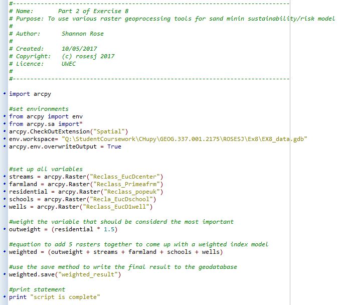
Frac Sand Mining Community Impact Model

The second part of this lab looked at the impact a frac sand mine would have on the community in the area it would be placed.  The mine would need to be far enough away from a stream as to no cause extra debris to end up in the water flow.  To assess this the centerlines, were used as the streams of concern because they represented the main flows of streams and rivers within the county.  Mines would have a high impact on a community if they were built on prime farmland.  It is not desirable to take away prime farmland to build a frac sand mine.  Frac sand mines need to be far enough away from residential areas due to the noise shed created by the mining operation.  A mine must be 640 meters away from a residential area according to standard zoning laws.  The National Land Cover Database was used to determine residential areas.  Any area labeled as developed was considered a residential area for the impact model.  A disadvantage of using this methodology is that industrial areas, commercial, and residential areas are not specified by using this methodology.  An advantage is that using this method of determining residential areas makes sure to encompass any form of developed area so that it can be guaranteed the 640 meters zoning law is followed, as to all developed areas are represented.  The same goes for schools, mining operations should be far enough away from schools as to keep schools a safe area and limit distractions the mining operation might cause for students.  The last factor that was assessed was wells, frac sand mining operations should occur far enough away from wells so that no water contamination occurs.  Figure 4 shows the ranking scale used during the reclassify operation for each raster.  The higher the rank value the less preferable that location is for frac sand mining due to the higher impact that location would have on the community. Figure 5 explains what ranking was given to each attribute within the various rasters used.      

Figure 4. Ranking scale used to assess

community impact a frac sand mining 

operation would have when 

reclassifying rasters.  

Figure 5. How rankings for the reclassification of rasters

were determined.

A model was created in model builder to demonstrate the workflow used to create the community impact model for frac sand mining locations in Trempealeau County. Much like the model in Figure 3, all datasets were converted to raster format and the Reclassify and Euclidean Distance tools were used to create the model. A viewshed was also created for a popular bike trail in Trempealeau County. The Viewshed tool determines the locations on a raster surface that can be seen from an input feature.  A DEM along with the bike path feature were used in the tool so that elevation could be taken into account when considering what might be visible from the bike path feature. The model that was created can be seen in Figure 5.  The Raster Calculator equation that was used added all of the rankings of the 5 rasters together.  The higher the output value the higher impact a mine would have on the community in that location.

Figure 5. Model builder model of the workflow used to create the
community impact model for frac sand mining in Trempealeau County.

Combining Models for Final Best Frac Sand Mining Locations 

The third part of the lab worked to combine the results of part 1 (suitability model) and part 2 (community impact model).  Figure 6 shows the ranking scale used during the reclassify operation for each raster.  The higher the rank value the better that location is for frac sand mining and the lower the rank the worse that location is for frac sand mining. Figure 5 explains what ranking was given to each attribute within the various rasters used.  Figure 8 is the model that was created in model builder to demonstrate the workflow used to create the final assessment of where frac sand mines should be placed in Trempealeau County.  The Raster Calculator equation that was used subtracted the community impact raster from the suitability raster.  The higher the output value the better the location is for a frac sand mine.

Figure 7. How the rankings for the reclassification of the
final raster assessment of frac sand mining operations were
determined. 

Figure 6. Ranking scale used to assess the
best locations to place frac sand mines when
reclassifying the final raster. 

Figure 8. Model builder model of the workflow used to create the final raster
assessment of the best locations for a frac sand mining operation in Trempealeau County.

Results and Discussion

The results of the suitability model determined that the west central part of the county is generally better for placing a frac sand mine.  There are more railroad terminals on the west side of the county.  The other factors considered are pretty evenly distributed across the county.  There is some discrepancy on the southern portion of the county.  The geology type there and landcover exclusion suggest the southern portion is not suitable for frac sand mining, but the slope and ground water depth suggest that this is a good location for a frac sand mine.  The results from the suitability model can be seen in Figure 9.

Figure 9. Results from the suitability model for Trempealeau County, WI.

The results of the community impact model determined that generally the western, northern and patches in the southeast part of the county would have a high impact on the community in these regions and not be suitable for mining operations. Schools, wells, and streams are highly concentrated in regions where the high impact was located.  The method for determining the residential areas might not have been the best method because most of the county was determined as a residential area when using the method that was used.  Prime farmland is scattered across the county and was not a huge determining factor on deciding the highest or lowest impact areas.  The results from the community impact model can be seen in Figure 10.

Figure 10. Results from the community impact model for Trempealeau County, WI.

The final results of this lab can be seen in Figure 11.  There are many possible locations to place frac sand mines in Trempealeau County.  There are some good places in the southern, southeast, and northwest portions of the county.  In the center of the county there are some patchy areas of good mining locations.  The worst locations for mining ended up being along waterways and water filled land regions on the southern boarder of the county.  There is also a bad location at a residential hot spot on the west side of the county.  

Figure 11. Final results for where to place a frac sand mine in Trempealeau County, WI.

Figure 12 shows a map showing the view shed from the Beauty & Diversity Abound bike trail on the east side of Trempealeau County.  A large portion of the land in this county can be seen from this popular bike trail.  Taking into account this prime recreational area and others could be added to the model for finding good locations for frac sand mines.  When people are at a pretty nature site, they would not want to see a large mining operation.

Figure 12. Viewshed from the Beauty & Diversity Abound bike trail in Trempealeau County.
A large portion of the county is visible from the loop this bike trail forms
on the east side of the county. 

Conclusions

This lab worked to find good locations in Trempealeau County, WI to place frac sand mines.  It is important to consider both land suitability and community impact factors when deciding where to place a frac sand mine.  This lab only looked at several factors that could be considered when locating a good location for frac sand mining operations.  There are many others that could be considered, like viewsheds from prime recreational areas, parks, or distance from wildlife areas.  The models made for this county could be adapted and used by other counties by using different raster data sets.  Also the models could be modified based on what characteristics the county finds important for considering different locations for frac sand mining operations.

Sources

GIS data. (n.d.). Retrieved May 16, 2017, from http://wghs.uwex.edu/maps-data/gis-data/.

Land Records. (n.d.). Retrieved March 10, 2017, from http://www.tremplocounty.com/tchome/landrecords/.

National Transportation Atlas Database- Bureau of Transportation Statistics. (n.d.). Retrieved March 10, 2017, from https://www.bts.gov/geospatial/national-transportation-atlas-database.

TNM Download. (n.d.). Retrieved March 10, 2017, from https://viewer.nationalmap.gov/basic/.

Web Soil Survey. Retrieved March 10, 2017, from https://websoilsurvey.sc.egov.usda.gov/App/HomePage.htm.

Lab 4: Network Analysis

Goal and Objectives There are three objectives in this lab:

This lab works to conduct a network analysis on the frac sand mining operations in the state of Wisconsin.  This lab is part of a multi part project to build a suitability/ risk model for sand mining in Western Wisconsin.  The focus of this lab was to use network analysis to better understand the impact heavy trucks moving sand from the sand mine location to the rail terminals has on the roads driven on.  In this lab first the route the sand takes from the mine to the closest railroad terminal was determined.  Next using simple calculations and estimates based on the number of truck trips and hypothetical estimates of costs of damage that occurs to the road per truck mile, the cost of damage that occurs to the roads per county was calculated.  The National Center for Freight and Infrastructure Research and Education has conducted research into similar methodology for determining road damage costs of frac sand trucks.  They have determined that road damage caused by these heavy trucks is a concern for many counties and local communities in Wisconsin.  The governments of numerous counties are looking into different methods for calculating the road damage caused by these trucks in hopes to recover the costs of damage from the mining operations.  This lab demonstrates one methods for calculating the costs accumulated by county from road damage.  The dataset that was used for the network analysis was the ESRI Street map USA.

There are three objectives in this lab:

1.  Use Pyscriptor to select mines based on the criteria that:
• The mine must be active
• The mine must not have a rail loading station on-site
• The mine must not be within 1.5 kilometers of a rail line
2. In Arc Map use Closest Facility solver in the Network Analyst toolbar to determine the closest rail terminal for each mine and the most efficient route that could be taken between the two
3. Build a model using Model Builder to automate the process of determining the closest facility route and the length of road being used by county. 
4. Calculate the cost per county that sand truck travel causes to the roads also using Model Builder

Methods

The first step of this lab was to use Pyscriptor to select mines that are currently transporting their frac sand from the mine to a rail terminal by using trucks to drive on local roads.  These types of mines must be classified as active, must not have a rail loading station on site, because that would eliminate any trucks driving on roads, and must not be within a 1.5 kilometer radius of the rail terminal, because if it is most likely a spur has been built again eliminating the need for trucks to transport frac sand. Mines that follow these criteria were selected for and exported as a new feature class in Pyscriptor using python coding.  The python script for this section of the lab can be seen in the Python Scripting post.

Next, in Arc Map the Network Analyst toolbar was used to determine the closest route a truck could take from a sand mine to a rail terminal using roads.  This route would most likely be the route taken by truck drivers to transport frac sand.  This was done by first selecting the rail terminals that use railroads from the rail terminal feature class.  This feature class included air terminals and other non-rail modes of transportation, which were irrelevant if railroads were not in use.  Using a  simple query statement to only select the terminals of railroads did this and the selection was exported as a new feature class.  Next, the network analyst extension was activated and ESRI original raw geospatial data on the streets in the United States was added to the Arc Map viewer.  The Network Analyst toolbar was added to the data frame.  The mine selection that resulted from the python script and the feature class of only rail terminals was added to the viewer.  A closest facility layer was added from the Network Analyst menu and the sand mines were loaded as the Incidents, and the rail terminals were loaded as the Facilities. The closest route from each mine to a rail terminal was generated.  Before model builder could be used to automate this process the feature class of selected mines generated by the python script were modified.  The Delete Field Data Management Tool was used to delete the address field, which can cause difficulties if left in the table when using Model Builder.

Next, a model in Arc Map was created using Model Builder to automate the processes used in this lab.  A toolbox was created in the geodatabase and the model builder was created inside that toolbox.  The previously described steps using the Closest Facility solver and the steps used to calculate the length of road used to transport sand by county and the estimated costs of damage caused by the sand transport were included in the model.  Figure 1 is of the model created in model builder.  The first 4 tools (Make Closest Facility Layer, Add Locations (2), and Solve) function as the operation of the network analysis using the closest facility solver described above.  This section results in selecting the most efficient road route from each mine to the nearest rail terminal.  The next two tools (Select Data and Copy Features) work to export the routes as a feature class.

The next section of tools in the Model Builder work to determine the total routes road length by county.  The Intersect tool was first used to create a geometric intersection between two feature classes, the selected routes feature class and a Wisconsin counties feature class. The features that overlap are included in the output feature class.  This allowed the road route lengths to be classified by county.  Next, the Project tool was used to project the new feature class that did not use decimal degrees as the form of distance measurement, but rather feet so that the actual physical length of the routes could be determined. Next the Summary Statistics tool was used to sum up the road length of the routes by county.  Following this step it is now known the length of road in feet used by trucks to transport frac sand by county.

Finally, the costs each county can expect to pay for road damage caused by the trips from the heavy frac sand truck routes was determined.  First, the Add Field tool was used to add a new field to the output table from the summary statistics used.  This field was for the road length in miles to make calculations easier by working with smaller numbers in miles instead of larger numbers in feet.  The next tool used was Calculate Field, used to populate the new field that was just created.  The algorithm used to populate this field was: (sum shape length)/5280, used to convert the length of road by county in feet to miles.  Next, another field was added to the table by using the Add Field tool.  This field was for costs in dollars of road damage.  The last tool used was the Calculate Field tool, which was used to populate the new field.  To calculate the cost per year a county should be expect to pay for road maintenance the following algorithm was used:
((road length * 2.2 cents) 100 trips)/ 100 = U.S. dollar amount costs of road maintenance a county will incur due to heavy sand truck traffic. The estimates that were used were that the hypothetical cost per truck per mile was 2.2 cents and that every year a mine would have a frac sand mine truck make 50 trips to and from the sand mine resulting on the road being driven on 100 times per mine.  The resulting table after this final step included the calculated road length in miles used by frac sand trucks and the cost of the damage in U.S. dollars that was caused by the trucks for each county.

Figure 1.  The model builder tool set that was used to complete this lab.  This tool set results in a table that gives the calculated length of road covered by a frac sand truck moving sand from a mine to a the nearest railroad terminal by county and the estimated costs each county will need to spend on road maintenance due to the heavy sand trucks driving these routes.  

Results and Discussion

The results of this study determined that out of the counties in Wisconsin with mines requiring frac sand transport from the mine to the rail terminal by the way of trucks driving on roads, the county that will have to spend the most money on road maintenance is Chippewa County at $613.22 per year.  The county that will spend the least amount of money each year on road maintenance is Winnebago at $2.12.  The calculated costs of the road damage by county can be seen in Figure 2.

For this exercise only the transport to railroad terminals was conducted or mines that the nearest rail terminal was in Wisconsin.  There was one mine in Wisconsin located in Burnett County, which is located very close to the Wisconsin boarder with Minnesota.  For this mine the closest rail terminal was located in Minnesota, so the road damage calculations were only included for what the county will incur, not what any Minnesota counties will incur in the completion of moving the frac sand to the final destination rail terminal.  

Figure 2. Table of the road length that is traveled by heavy frac sand trucks and the cost of road maintenance by county.

In Figure 3. agraph can be seen which shows the extent of the cost and road length differences between frac sand truck transport impacted counties in Wisconsin.  It can be seen how Chippewa County is acquiring nearly double what most other counties are paying inroad damages.    

Figure 3. Graph for visualizing the comparison between the road length and the cost of road maintenance distributed through effected Wisconsin Counties. 

The three counties with the most damage costs due to truck frac sand transportation are Barron, Chippewa, and Eau Claire counties.  This is interesting given that the top three counties with the largest number of mines with sand being transported are Chippewa, Trempealeau, and Eau Claire.  Barron only has 4 mines that are having frac sand transported by trucks and Chippewa has 6 mines.  Trempealeau has 10 mines, the greatest number of mines transporting sand this way and it is not ranked as having the greatest cost of road damage.  This is interesting given Trempealeau County is not paying nearly as much as Chippewa County is and Trempealeau has 4 more mines than Chippewa.  It can also be seen that Barron County sends all of its trucks to Chippewa County for the nearest rail terminal, this is a possible explanation for Chippewa's increased damage costs.  Also Chippewa County is a larger county than Trempealeau leading to longer road distances to be traveled to transport frac sand.

Figure 4. Map of the roads used to travel between frac sand mines and railroad terminals including the costliness of the damage to the roads due to the transport.

There were a few estimates and hypothetical situations utilized in this lab.  These make the results of the lab not exact and should be modified if this model were to be used to generate actual data for a real analysis.  These estimated include that the cost of damage caused by a truck per mile was estimated at 2.2 cents and the number of truck trips 100 per year number was used as an estimate.  Also the routes that were determined to be the routes the frac sand trucks would take were only calculated as the nearest rail terminal to the sand mine and the roads used were just the most efficient routes.  The trucks might use different terminals given unknown circumstances like the size of the terminal and how many mines it can service.  The trucks might also use different road routes given unknown circumstances like road closures, changing the effected roads and changing the pricing per county.  Also the size of the mine was not taken into account, a larger mine would most likely require more truck trips, or the weight of the truck loads would be greater causing an increased amount of damage to the roads that those trucks are driving on.

Conclusions

Overall, the methodology used in this lab was sound for determining the routes potential frac sand tucks would take between a frac sand mine and the nearest rail terminal and the cost of road damage that a county would incur per year based on the length of the road traveled by the trucks within that county.  The network analysis tool is very versatile and easy to operate.  There are many operations it can conduct outside of just using road networks; water and utility networks can also be examined.  The Model Builder that was created in this lab can be used to calculate the inquires for a different state given a different mine dataset and if correct pricing and trip counts were used this model could be used to accurately calculate the expense of road damage per county, instead of just using estimates that were used in this lab.  

Sources

National Center for Freight and Infrastructure Research and Education. (2013). Transportation Impacts of Frac Sand Mining in the MAFC Region: Chippewa County Cause Study. Retrieved from http://midamericafreight.org/wp-content/uploads/FracSandWhitePaperDRAFT.pdf.

Lab 3: Data Normalization, Geocoding, and Error Assessment Sand Mining Suitability Project

Goals and Objectives

The goal of this lab was to use the ArcMap geocoding capabilities to geocode the locations of 19 sand mines in Wisconsin and compare my results with the actual locations.  This lab is a part of a multi part project to build a suitability/ risk model for sand mining in Western Wisconsin.  The focus of this lab is to work with normalizing raw data, geocode several addresses, and compare the geocoding results.  There are 128 sand mine locations in the state of Wisconsin according to the downloaded DNR data.  To reduce workload, each student in the class was randomly assigned 19 mines.  Each individual mine was assigned to 4 people to compare results.    

There are five objectives for this lab:

1. In an Excel table normalize the address data for sand mines in Wisconsin
2. In ArcMap connect to the ESRI geocoding service and geocode the assigned 19 mines
3. Using the department ArcGIS server add the Public Land Survey System (PLSS) feature class
4. Manually locate all 19 mines that use PLSS locations
5. Compare personal results with those of classmates and the actual locations from given coordinates from the DNR.

Methods

Data Normalization
When the excel data table of the addresses of sand mines in Wisconsin was downloaded from the DNR website the address data table was found to not be normalized.  The first step of this lab exercise was to normalize the address data table for the 19 mines to be completed.  Data normalization is a refinement process that organizes data into columns within in a table in order to reduce redundancy and ensure data integrity.  For the normalization of the excel table downloaded from the DNR, the main element that was normalized was the address column of the downloaded table.  The downloaded data address column appeared with many address components all in one column: house number, street name, street type, city, state, and postal code.  Through data normalization most of these components were broken apart into separate columns within the table separating out city, state, and postal code so that address matching may be more accurate.

Geocoding
After the address data was normalized, in ArcMap the geography department enterprise ArcGIS server account was connected to and the assigned 19 mines were geocoded.  A map was added to the viewer to assist with geocoding the mines.  First ArcGIS online had be logged into using the university's enterprise account.  The excel sheet with the 19 mine addresses or PLLS locations was added to the viewer.   Two processes of geocoding were used.  First geocoding was conducted through using an address locator, the geocoding tool bar was turned on and the Geocode Address option was selected.  The World Geocode Service was selected and the excel sheet was selected.  The proper fields were set for geocoding to match with the different fields within the excel sheet.  The geocoding process was conducted after this process was complete.  Once the geocoding addresses function was complete a window, Figure 1, was opened providing information on how well the geocoding process conducted the matching of addresses.  There was only one address that could not be matched.  This method of matching, by using the address locator works well for addresses that have street addresses, this method does not match Public Land Survey System (PLSS) addresses.  The unmatched address were inspected and it was indeed a PLSS address.  This method does not work for addresses with PLSS locations.

Next the second process of geocoding was used, geocoding based on PLSS locations.  A database connection was added in ArcMap to the WiDNR2014 server.  This allowed access to the townships and sections feature classes to interpret PLSS locations.  Both shapefiles were added to the viewer.  Using the Address Inspection function of the geocoding toolbar and each address was assessed for accuracy by using the zoom to candidates function in the Interactive rematch window.  Each geocoded location was checked against the base map, if a map was not where the location was specified the PLSS location was found and the new address was picked from the map.  PLSS locations were found by using the township shapefile to locate the North or South component and the sections shapefile to locate the East or West component.  All addresses that were geocoded in this case were moved at least a little bit.  The address for each mine was placed at the driveway from a major road to the mine.  None of the geocoded addresses appeared in this correct location.  Once all addresses were properly located.  The feature class containing all of the geocoded locations was saved and exported as a shapefile.  

Figure 1. Geocoding addresses matching report.

Compare to Fellow Classmates Results
Following the completion of geocoding the 19 mines, the class combined their results allowing for students to compare their individual geocoded result with that of their classmates.  The Wisconsin State Cartographers office requires a local accuracy at a 95% confidence interval.  It was decided to assess if these standards could be upheld by checking for the accuracy of each of the 19 geocoded mines.  To begin all of the shapefiles of geocoded mines of students who submitted their mines for comparison were added to the ArcMap window.  Out of a class of 27 students only 16 students submitted their geocoded locations for comparisons.  Because of this a full comparison could not be collected, there was some data missing.  First all of the shapefiles were merged by using the Merge analysis tool.  Next the data table that contained all of the merged addresses was checked for merge accuracy.  the Mine Unique ID field was the most important.  If any of the mines did not have their IDs in this correct field the editor toolbar was used to manually move the IDs to the same correct field.  Next, both the shapefile containing my geocoded mines and the shapefile containing all of my fellow student's geocoded mines were projected to the same coordinate system not measured in decimal degrees, but an actual physical distance measurement.  A coordinate system measured in feet was used.

Next, the Point Distance analysis tool was used to determine the distances from input point features to features from a different feature class called near features within a specified search radius.  This tool was selected because it could not be assumed that the closest point would represent the correct mine, within this data set there are many sand mines close together in Western Wisconsin.  My georeferenced points were used as input point features and the classmates merged georeferenced locations point feature class was used as the near features.  No search radius was specified because the size of the distance between the two points could vary in size.  After the tool finished running the attribute table of the feature class containing all of the merged student's mines was exported as a table.  In this exported table all fields were deleted using the Delete Fields tool except for the Mine Unique ID field. This table was then joined to the output table of the point distance tool by matching the Near FID and the Object ID fields.  This allowed for the Mine Unique IDs to be compared to determine the distance between my mine geocoded location and that of other students.  The distances that separated each of the 19 geocoded mine locations and other students were recorded in an excel table, Figure 4.

Compare to Actual Mine Coordinate Locations
Also the exact location of each mine was given to the class from coordinate data that was exempt from the originally supplied DNR downloaded data but was acquired in the download.  This data was compared to the student's 19 georeferenced points.  This was done by first projecting the two feature classes to the same coordinate system that was not in decimal degrees so that distance could be calculated.  Next, the Point Distance tool from the Analysis toolbox within the proximity toolset was used.  This tool determines the distances from input point features to features from a different feature class called near features within a specified search radius.  This tool was selected because it could not be assumed that the closest point would represent the correct mine, within this data set there are many sand mines close together in Western Wisconsin.  The georeferenced points were used as input point features and the exact location point feature class was used as the near features.  No search radius was specifies because the size of the distance between the two points could vary in size.  After this tool finished running an output table resulted comparing each input feature ID to every near feature ID resulting in the distance separating the two points.  The correct ID's were cross referenced for their coordinating Unique Feature Mine ID and then the correct ID's were searched for the right combinations that resulted in comparing the same points between the two feature classes.  The distance that separated each of the 19 points were recorded in an excel table, Figure 5.   

Results

Below can be seen the data table without normalization (Figure 2) and the data table with normalization (Figure 3).  The main difference can be seen in how the addresses are recorded.  The normalized addresses have different fields for each component of the address and the addressed without normalization has the whole address lumped together in one field.

Figure 2. Data table without normalization.      Figure 3. Data table with normalization.

Below are the distance comparisons between my geocoded mine locations and the geocoded locations of my classmates (Figure 4), and my geocoded mine locations and the actual coordinate locations of the mines (Figure 5). 

Figure 4. Distance comparison between my geocoded mine locations and the geocoded locations of my classmates. 

Figure 5.  Distance comparison between my geocoded mine locations and the actual coordinate locations of the mines.

Below is a map with my estimates of mine locations, my classmates estimated mine locations, and the correct locations of the mines (Figure 6).    

Figure 6. Map comparing the locations where my classmates estimated mine locations to be, the correct mine locations, and my estimates of mine locations.  The mine unique IDs have been labeled.

Discussion

Most of my geocoded mine locations were generally correct.  My data did not meet the 95% accuracy upheld by the Wisconsin State Cartographers office, there were many more errors than I thought there would be.  There were several errors that resulted in the distances of the sampled value from the actual value of the points of the sand mines in Wisconsin. There were many different types of errors that were encountered include inherent and operational errors.  Inherent errors are errors that occur as a result of the spatial nature of geographic data.  Operational errors are errors that occur during the operation of the procedures for collecting, managing, and using geographic data.  There were three mines that had significantly greater amount of error, mines 208, 229, and 289.

The inherent errors that occurred include attribute data input error.  The addresses in the original DNR downloaded dataset might have been incorrect.  The addresses could have been jumbled by the DNR during data input.  I think this is the error that occurred for mine 208.  Mine 208 did not have a PLSS location, just a street address.  The geocoded address should have been more correct.  There might have been an error in entering the street address in comparison to the coordinate locations on the part of the WI DNR.  Mine 229 might have been an inherent error as well.  The PLSS location of the coordinate correct location is different from the PLSS location that was downloaded and used for the geocoding.  This would be an error on the part of the WI DNR in not entering in the correct data. The same goes for mine 289, the downloaded data recorded the mine was in township 24 North but the coordinate location has it in township 25 North.

Operational errors accounted for more of the smaller errors in distance.  The operational errors that occurred include the fact that there were a few mines where there were multiple mines near each other and in the same PLSS area where I chose a different mine instead of the correct one.  An example of this was found for mine 250 where there were multiple mines in one location.  My mine geocoded locations were more closely related to the mine locations of my classmates than the correct mine locations.  I attribute this to the fact that the class received instructions telling us general rules for where to place our geocoded location points, where the driveway to the mine meets a major road, or the main entrance to the mine.  The coordinates of the correct location of the mine were generally to the center of the mine.  An example of this was mine 202 where the correct coordinate location was at the center of the mine and mine and my classmates geocoded location was at the end of the driveway to the mine.  Another example of this error during geocoding there were a lot of decisions made by the user, where to exactly place the geocoded point, which entrance to the mine appears as the main entrance if there were multiple entrances, making error a very possible reality.  Something that could have prevented errors is the addition of protocols for data normalization and how data tables should be organized.  This error occurred when merging datasets, when users normalized their tables some changed the names of the columns causing trouble during merging and fields within tables were could not be matched and merged correctly.

We can know which points are correct and which are not by using the latitude and longitude values supplied by the DNR.  This data is the most accurate data in use, but errors could be present within this dataset from the process of collecting this data in the field.  The only way to know if the coordinates are correct is to go to the coordinate location and see if there is a sand mine located there.

Conclusion

Throughout this lab many important lessons about the complicated process of geocoding and the inaccuracies that can arise were learned.  It is important to be aware that errors may exist in datasets and may have an impact on the final outcomes of a project.  Error could have been minimized if normalization protocols were set in place and specific protocols for where geocoded points should be placed in reference to the location of the mine were in place.  Ultimately errors always exist in datasets and are an unavoidable reality, but being able to minimize errors to acceptable standards and being able to recognize that data errors will occur are important skills.

Lab 2: Gathering Data for Sand Mining Suitability Project

Goal

To become familiar with downloading data from different data source websites on the internet.  After downloading the data sets, the data will be imported into ArcGIS, joined with other data sets, and projecting each data set to the same coordinate system.  In completing the lab, a geodatabase will be created to store the data.  

This lab serves as the beginning of a several part project that works to create a sustainability/risk model for sand mining in Western Wisconsin.  Trempealeau County is the Wisconsin county that is the main study area for the research.

Objectives

There are four different objectives associated with this lab.

1. Download data from several data source websites
2. Importing downloaded data, joining tables, merging data, and viewing the data
3. Creating a Python script that projects, clips, and load all of the downloaded data into a geodatabase
4. Creating a few maps to display the data collected and organized for the project

Methods

Data files were downloaded and unzipped from a number of different websites.

US Department of Transportation
(https://www.rita.dot.gov/bts/sites/rita.dot.gov.bts/files/publications/national_transportation_atlas_database/index.html)

The 2015 National Transportation Atlas Database (NTAD) was downloaded.  This database includes a nationwide set of databases of transportation facilities, transportation networks, and other transportation associated utilities.

USGS National Map Viewer
(https://viewer.nationalmap.gov/basic/)

The 2011 National Land Cover Database (NLCD) was downloaded.  This database includes a raster of a selected area of interest symbolized by land cover type.  Trempealeau County is covered by fifteen different land cover types.

The Elevation Product of a 1/3 arc-second DEM was also downloaded.  Two DEMs had to be downloaded because Trempealeau County falls within the two downloadable DEMS.  These DEMs were downloaded as raster datasets.     

USDA Geospatial Data Gateway
(https://datagateway.nrcs.usda.gov)

The Land Cover Cropland data layer (NASS) for Trempealeau County was downloaded.  The database included a raster of the area of interest symbolizing the land cover by crop type.  In Trempealeau County forty-one different crops were symbolized.    

Trempealeau County Land Records
(http://www.tremplocounty.com/tchome/landrecords/)

The Trempealeau County GIS file geodatabase (TMP) was downloaded.  This geodatabase consists of feature classes containing data pertaining to boundaries, transportation, recreation, land, emergency, and cadastral data.  The transportation records from the NTAD is more up to date and will be used in this project instead of the TMP transportation datasets.

USDA NRCS Web Soil Survey
(https://websoilsurvey.sc.egov.usda.gov/App/HomePage.htm)

The NRCS Soil Survey was downloaded for Trempealeau County.  Included in the download was shapefiles of soil data and database containing many personal geodatabase tables containing soils data.

Data Accuracy

The metadata for each data source was consulted to complete the following table on data accuracy.

*This was a downloaded geodatabase, so each data source comes from a different specific location.  For specific information on the data from a certain feature class see 

http://www.tremplocounty.com/tchome/landrecords/data.aspx  for links to individual metadata.   

Data Accuracy Conclusions

It was rather difficult to determine the different data accuracy for the various data sets.  Metadata is not easy to read and a lot of data accuracy information was missing.  The lack of information was not consistent amongst the data sets, some had more missing than others.  The metadata of the NLCD stated that "a formal accuracy assessment has not been conducted".  Also some sources admitted some accuracy data is "unknown".  This seems concerning and should be noted as working through this project that there is probably some error present in the data.    

Maps

The maps created displaying the datasets that had python scripting applied to them to project and clip the datasets.

Figure 1. Map displaying the DEM, NASS, and NLCD data after python scripting was applied. 

Sources

Land Records. (n.d.). retrieved March 10, 2017, from http://www.tremplocounty.com/tchomr/landrecords/.

National Transportation Atlas Database | Bureau of Transportation Statistics. (n.d.). Retrieved March 10, 2017, from https://www.rita.dot.gov/bts/sites/rita.dot.gov.bts/files/publications/national_transportation_atlas_database/index.html.

TNM Download. (n.d.). Retrieved March 10, 2017, from https://viewer.nationalmap.gov/basic/.

USDA:NRCS:Geospatial Data Gateway. (n.d.). Retrieved March 10, 2017, from https://datagateway.nrcs.usda.gov/.

Web Soil Survey. Retrieved March 10, 2017, from https://websoilsurvey.sc.egov/App/HomePagehtm.

Python Scripting

What is Python?

Python is a programming language that is widely supported.  This language can be applied to data analysis, conversion, management, and map automation.  This free and open-source language has been accepted as the official scripting language for ArcGIS geoprocessing.  ESRI has fully embraced the Python scripting language.  Some advantages of Python include that it is easy to learn, it can be easily scaled to project size, it is applicable across platforms, it is embedded allowing ArcGIS to be scripted, it is stable, and can be utilized by a large community of users.

Why learn Python?

Python is a well accepted scripting language that is widely applicable.  If using ArcGIS in the future, it is important to be familiar with Python scripting, as it is an important skill to have that increases productivity.

Scripts

Lab 2: Gathering Data for Sand Mining Suitability Project 

Python script written to project, clip, and load all of the data for the project into a geodatabase.

Figure 1. Screenshot of script written in Pyscripter.

Figure 2. Screenshot of results of script in Pyscripter.  The script was successful.

Lab 7: Network Analysis

Python script written to select only active mines that do not have a rail loading station on site and are not within a 1.5 kilometer distance of a railroad.  This project aims to calculate the impact of trucking sand from mines to rail terminals on local roads, if a mine site uses a railroad for transportation, then it is not having an impact on the damage to roads because it does not use trucks.  

Figure 3. Screenshot of script written in Pyscripter. 

Figure 4. Screenshot of results in Pyscripter.  The script ran successfully. 

Lab 8: Raster Modeling

Python script written to to generate a weighted index model for the sand mining risk model that was created in Lab 8.  In this script raster math was done, and the factor of residential was seen as the most important factor so it was weighted by a factor of 1.5 when added to the other factors.  Residential was selected as the most important factor because residential represents the rankings for the land areas closest to residential areas as highest risk and the areas farther away as the lowest risk.  This is important for managing the impact of the noise shed created by the mining operation.  Keeping the locals happy is very important in conducting a mining operation, so making sure the mines were far enough away from residential areas was weighted as more important than the other factors.  The raster math conducted added all of the raster factors, streams, farmland, schools, wells, and the weighted residential together to conduct the risk model of the ranked rasters.  The locations with the highest values are the most at risk and the locations with the lowest values are of the least risk.  This script runs much like a Raster Calculator tool would in ArcMap.          

Figure 5. Screenshot of script written in Pyscripter.

Figure 6. Screenshot of results in Pyscripter.  This script ran successfully. 

Sources

ArcGIS Help 10.2, 10.2.1, and 10.2. (n.d.). Retrieved March 09, 2017, from http://resources.arcgis.com/en/help/main/10.2/index.html#//002z00000001000000

Lab 1: Sand Mining in Western Wisconsin Overview

What is sand frac mining?

Sand frac mining also called "fracking" or hydraulic fracturing is a process where frac sand is suspended in a liquid and infused into gas and oil wells in fractured of the earth at a very high pressure.  This high pressure breaks open fractures even more and causes new fractures to form this allows for gas and oil to be more easily extracted.  Frac sand is nearly pure quartz sand of a particular size and shape that must be well rounded and extremely hard of a uniform size to be used for sand frac mining.  Before shipping the frac sand to the mining work site the sand undergoes a process of is being washed and dried.  The sand is also checked for uniformity, and the usable sand is not sent to the mining site.


Where is sand frac mining in Wisconsin?

The states with the most frac sand mining include, Wisconsin and Minnesota.  Wisconsin controls 75% of the frac sand market in the United States today.  In Wisconsin sand frac mining is currently taking place in the sandstone formations of western and central Wisconsin.  Due to several of Wisconsin's geologic formations being located near the surface and the sand meeting specified qualifications for frac san mining, Wisconsin is known for having some of the best frac sand in the country.

Figure 1. A map of the sandstone formations and active or developing frac sand mines and processing plants in Wisconsin.  Map from the Wisconsin Geological and Natural History 2012 Survey (Frac Sand in Wisconsin).    

What are some of the issues associated with sand frac mining in Western Wisconsin?

Some of the issues with sand frac mining in Western Wisconsin include, transportation routes for the frac sand.  Roads need to be upgraded and receive routine maintenance that are apart of the sand haul routes.  It is difficult for truck drivers to know which roads and be driven on and which counties or states have which restrictions for hauling sand.    

Other concerns with frac sand mining include water and air pollution as well as endangering public health.  The sand frac mining operations in Wisconsin are run without many regulations that account for environmental impacts or public health.  Frac sand mining impacts the earth and the residents of Wisconsin by exposing locals to airborne particulate matter which damages lungs, chemicals are damaging surface waters, and communities are being exposed to these toxic chemicals as well.  Also agriculture suffers by endangering the productivity of soils and ground water reserves and drawn down.  Wisconsin laws regarding these issues are not taking into account the rapid growth of this industry.  

Frac Sand Mining in the News:

Currently many local communities are working to stop frac sand mining or to prevent new mines from being installed.  In Jackson County, Wisconsin local families have sued the AllEnergy Hixton as an attempt to stop them from opening a 750-acre mine.  Their defense to the lawsuit is that the mine will create a lot of dust, noise, light, and blasting that will disrupt their lifestyles and decrease their property values.  The fault on the project is causing it to loose money everyday.  Financing to continue the project cannot be secured until the lawsuit is over.  The mining project has all required permits and can begin the mining process as soon as the financing is finalized.  The case is caught up on that AllEnergy is being sued over fictitious damages; the mine still hasn't been created.  The case is expected to go to the court of appeals over if the mine can be in a lawsuit if it has yet to do any damage.  This is a current example from February 10, 2017 that highlights the controversy and fear over the damages frat sand mines can cause. 
How can GIS be used to further explore some of these issues?

In the United States numerous states and counties have enacted suspensions of frac sand mining until the extent the mining has on water supplies, public health, safety, and transportation infrastructure has been improved.  GIS can be used a useful tool in working on all of these concerns.

GIS can be used to create a database or map of what roads local governments allow sand trucks to drive on and that can be updated to show road qualities.  The map can include which roads require maintenance and should not be driven on.  The case study on frac sand mining highlighted that it can be difficult to keep track of county and state justification across states, this can be easily done in GIS by setting up proper rules and restrictions within feature classes.  Trains are also being used to transport sand; rail lines can be mapped using GIS as well.


Citations:

Case Study on Impacts of Sand Mining

http://midamericafreight.org/wp-content/uploads/FracSandWhitePaperDRAFT.pdf

Frac Sand Mining. (n.d.). retrieved March 01, 2017, from http://conservationvoters.org/issues/frac-sand-mining/

Frac Sand Mining Fact Sheet
http://wcwrpc.org/frac-sand-factsheet.pdf

Hopeful frac sand operator seeks to boot court challenge. (2017, February 10). Retrieved March 01, 2017, from http://lacrossetribune.com/news/local/hopeful-frac-sand-operator-seeks-to-boot-court-challenge/article_dd921326-4020-5f18-b692-2ee17a94bb7d.html